Data Science Lifecycle und Visualisierung
Unit 1
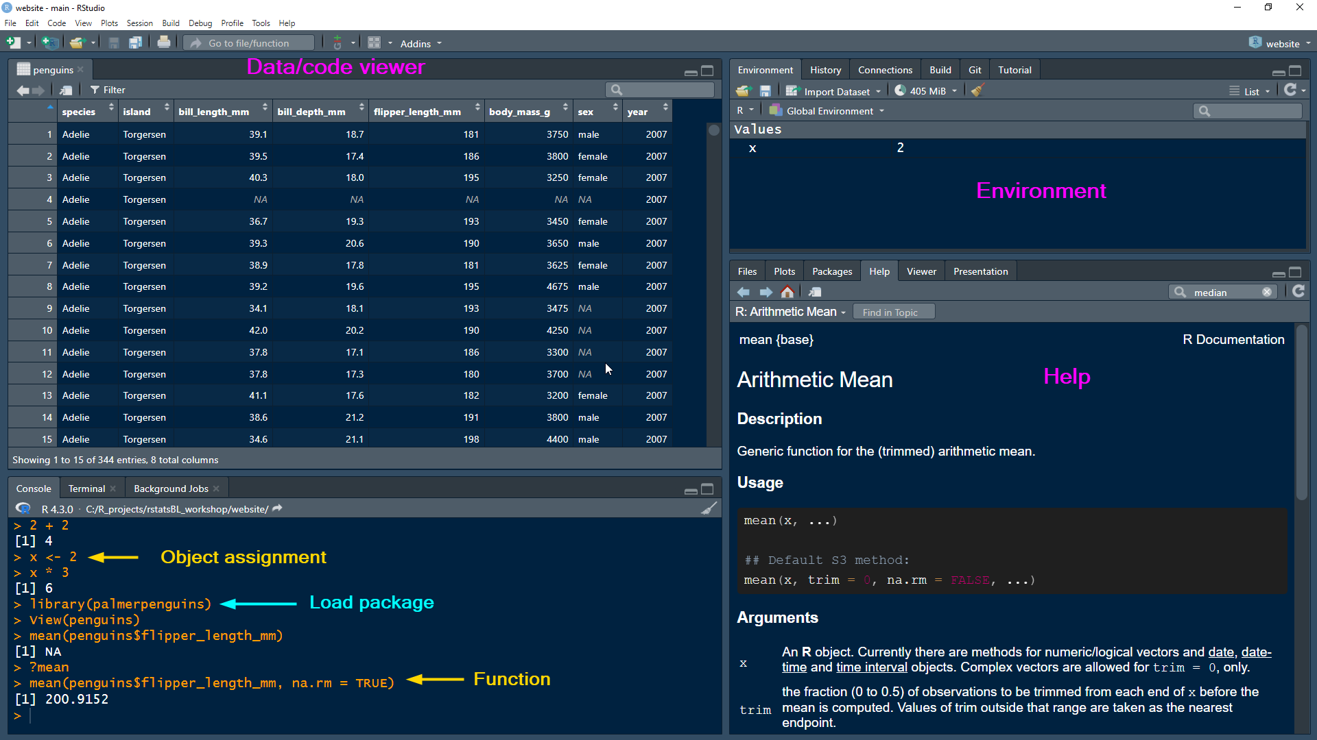
Hallo R! 👋
RStudio
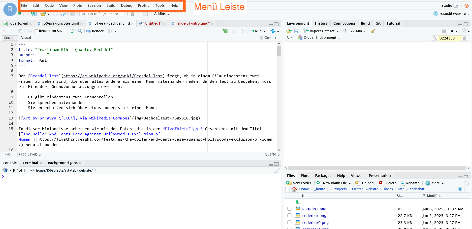
RStudio
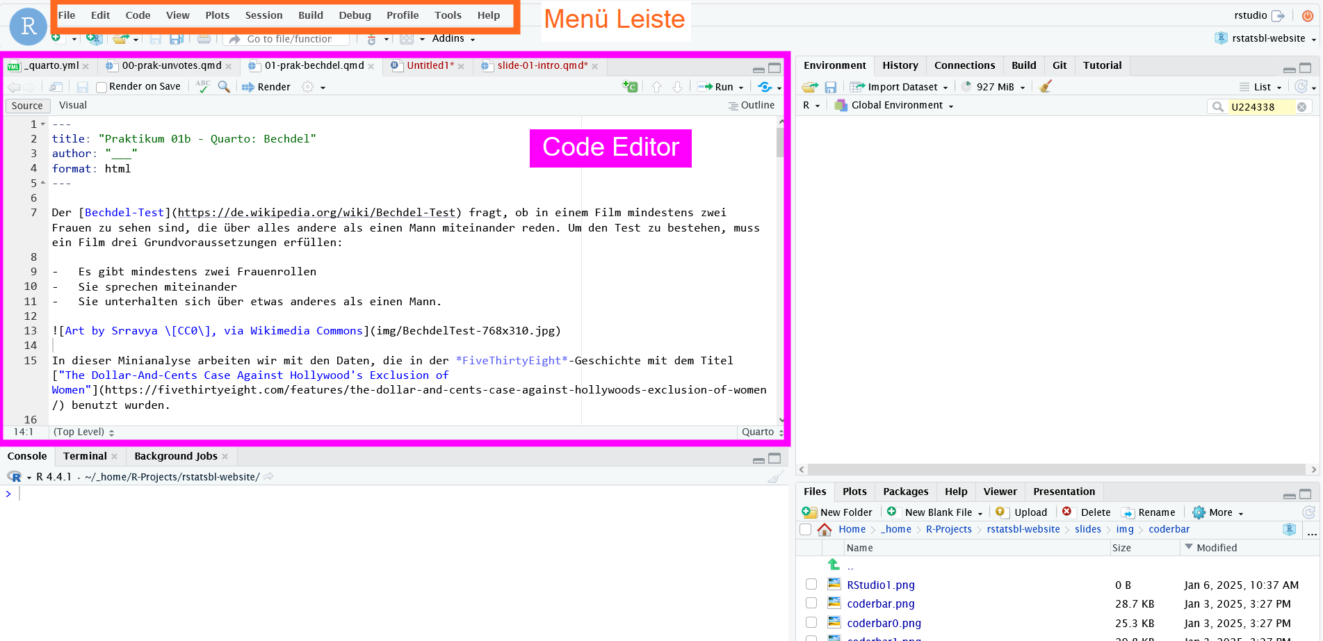
RStudio
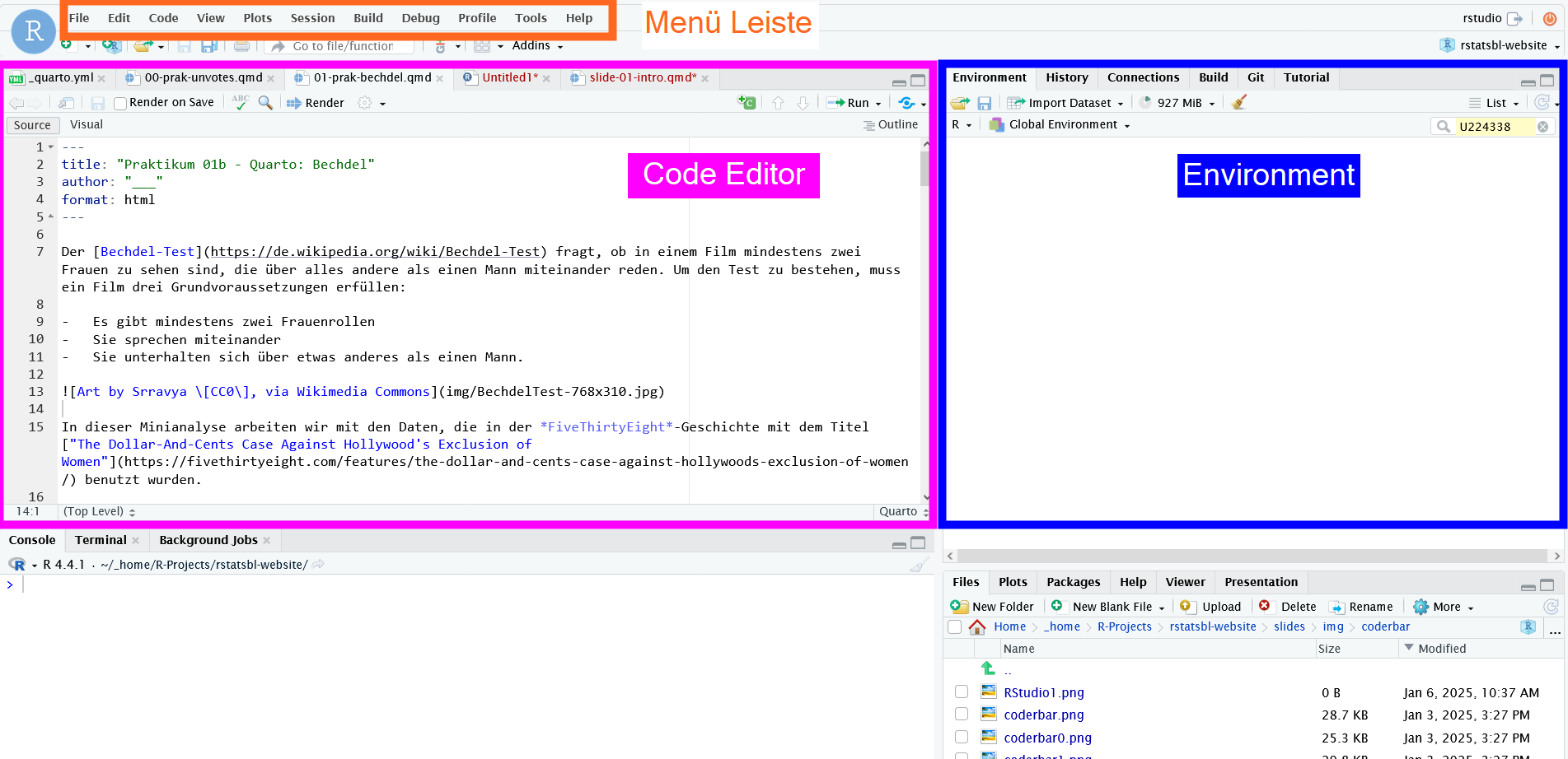
RStudio
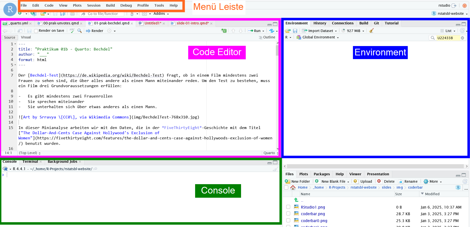
RStudio
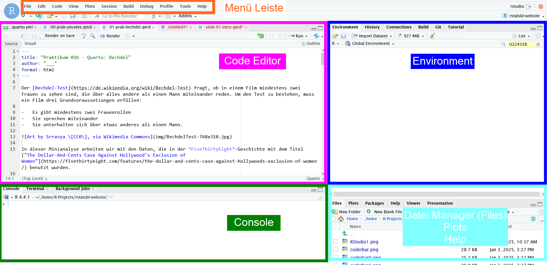
RStudio und R-wesentliches
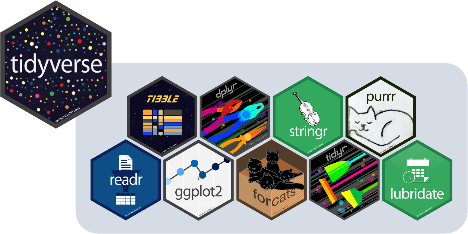
Tidyverse
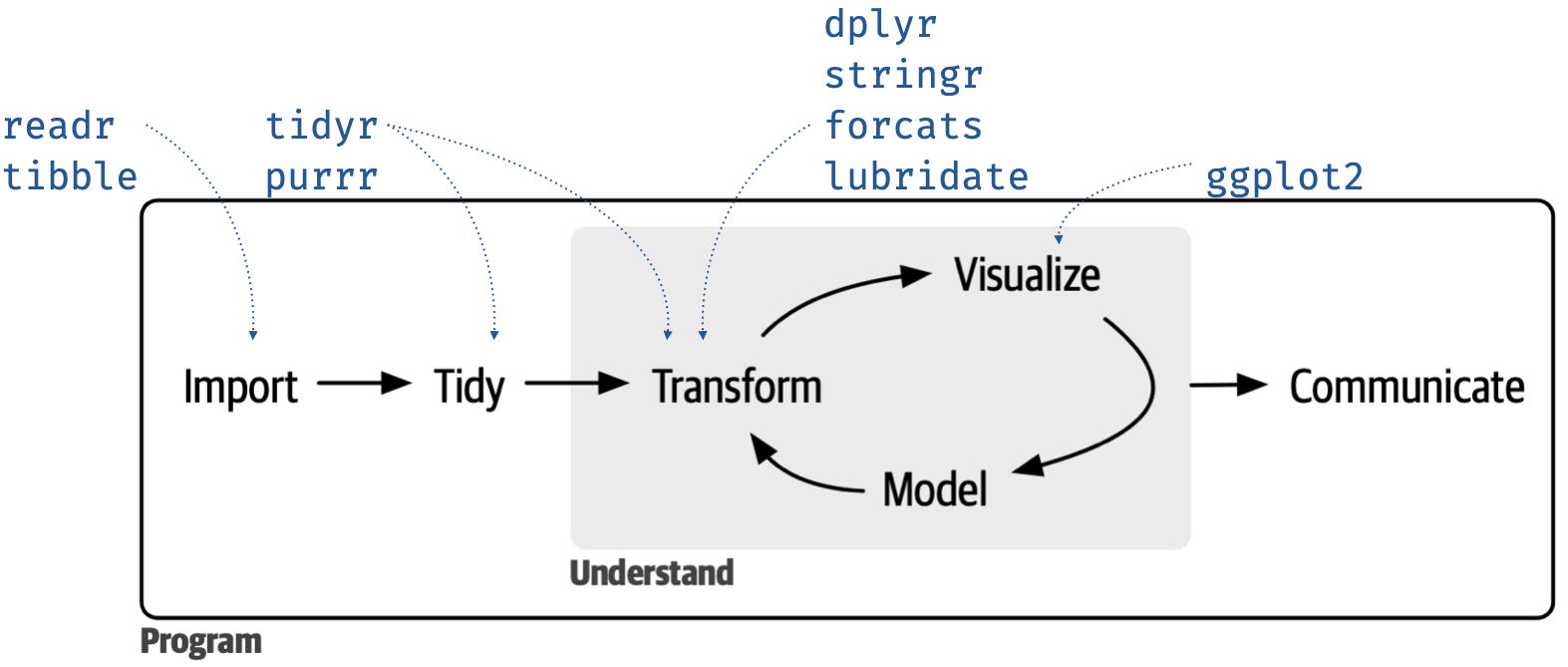
Data Science Lifecycle
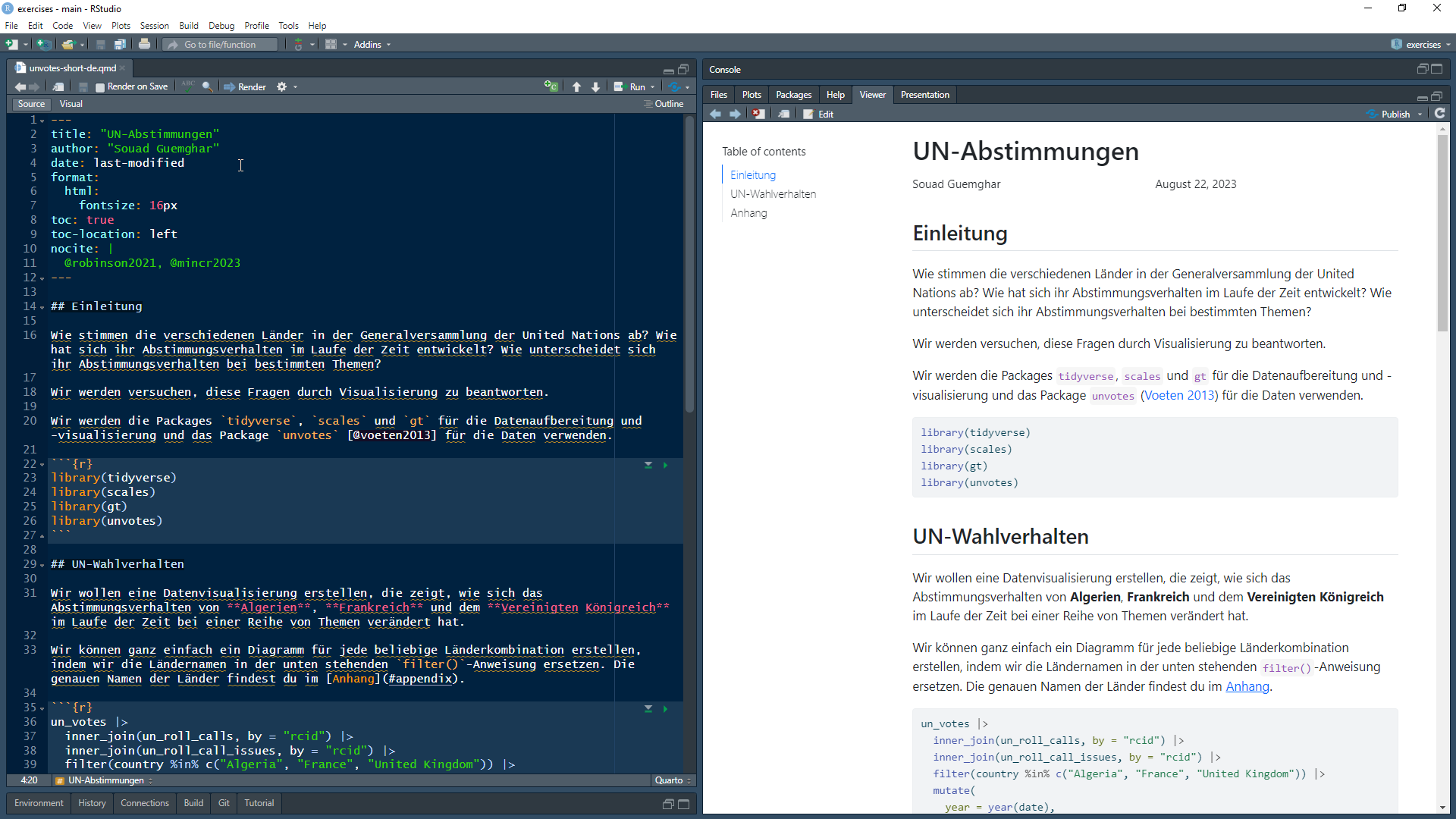
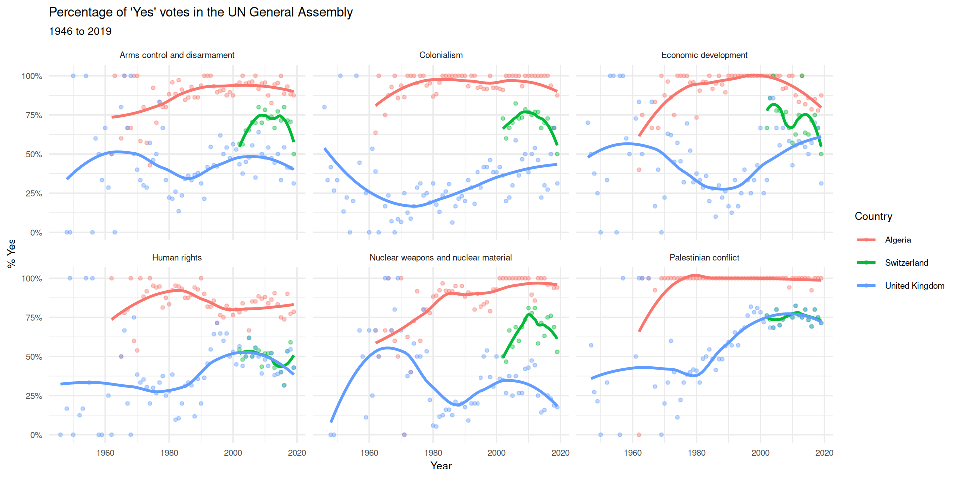
```{r}
#| code-line-numbers: "|5-7|8|16|22"
#| eval: false
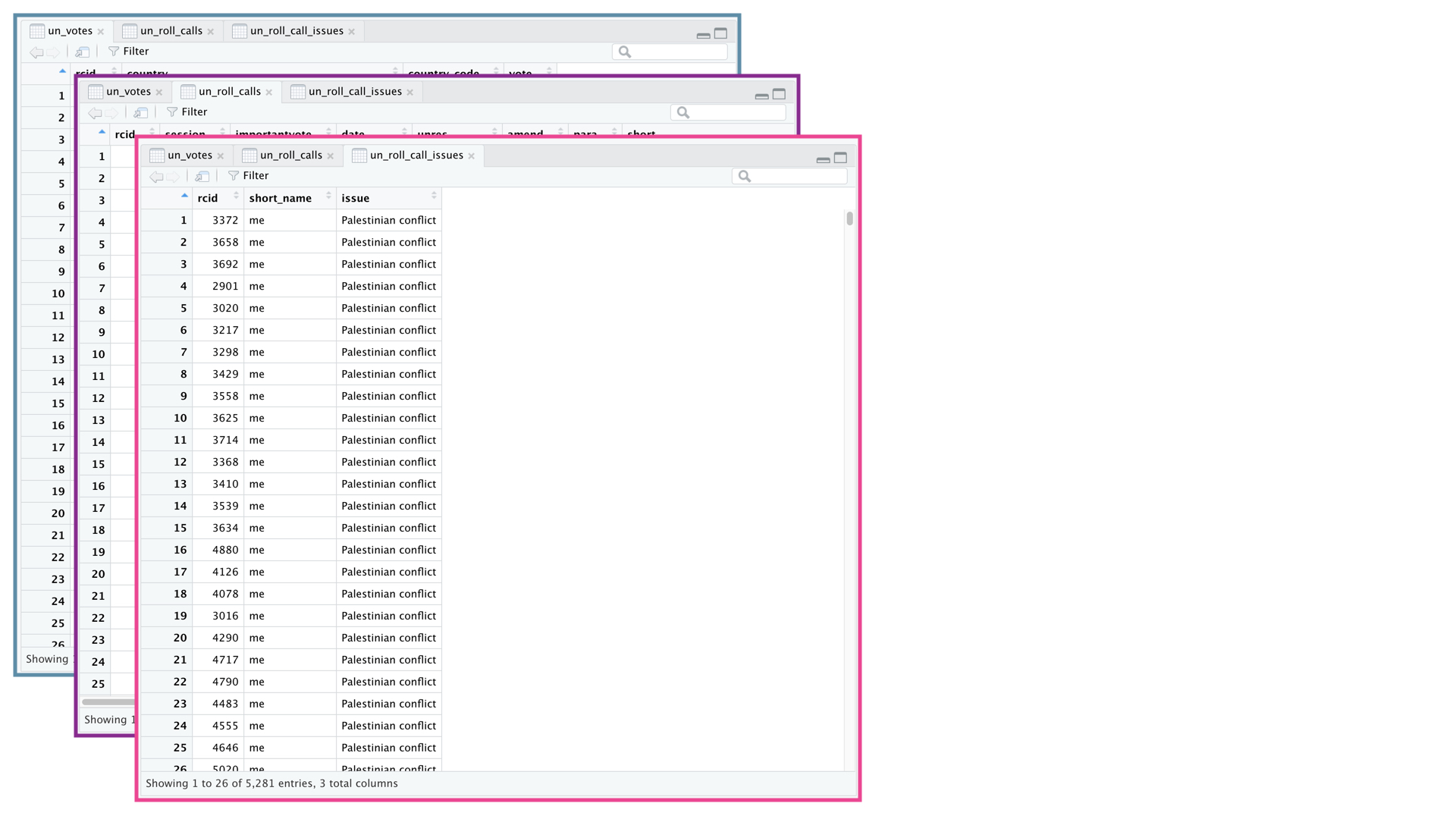
un_votes |>
inner_join(un_roll_calls, by = "rcid") |>
inner_join(un_roll_call_issues, by = "rcid") |>
filter(country %in% c("Algeria", "Switzerland", "United Kingdom")) |>
mutate(
year = year(date),
issue = fct_relevel(issue, "Arms control and disarmament"),
issue = fct_relevel(issue, "Palestinian conflict", after = Inf)
) |>
group_by(country, year, issue) |>
summarise(percent_yes = mean(vote == "yes")) |>
ggplot(mapping = aes(x = year, y = percent_yes, colour = country)) +
geom_point(alpha = 0.4, size = 1) +
geom_smooth(method = "loess", se = FALSE) +
facet_wrap(~issue) +
scale_y_continuous(labels = label_percent()) +
labs(
title = "Percentage of 'Yes' votes in the UN General Assembly",
subtitle = paste(un_roll_calls |> summarise(min(year(date))) |> pull(), "to", un_roll_calls |> summarise(max(year(date))) |> pull()),
colour = "Country",
x = "Year",
y = "% Yes"
) +
theme_minimal() +
theme(
text = element_text(size = 8)
)
```
R Package ggplot2
R Package ggplot2
Rows: 344
Columns: 8
$ species           <fct> Adelie, Adelie, Adelie, Adelie, Adelie, Adelie, Adel…
$ island            <fct> Torgersen, Torgersen, Torgersen, Torgersen, Torgerse…
$ bill_length_mm    <dbl> 39.1, 39.5, 40.3, NA, 36.7, 39.3, 38.9, 39.2, 34.1, …
$ bill_depth_mm     <dbl> 18.7, 17.4, 18.0, NA, 19.3, 20.6, 17.8, 19.6, 18.1, …
$ flipper_length_mm <int> 181, 186, 195, NA, 193, 190, 181, 195, 193, 190, 186…
$ body_mass_g       <int> 3750, 3800, 3250, NA, 3450, 3650, 3625, 4675, 3475, …
$ sex               <fct> male, female, female, NA, female, male, female, male…
$ year              <int> 2007, 2007, 2007, 2007, 2007, 2007, 2007, 2007, 2007…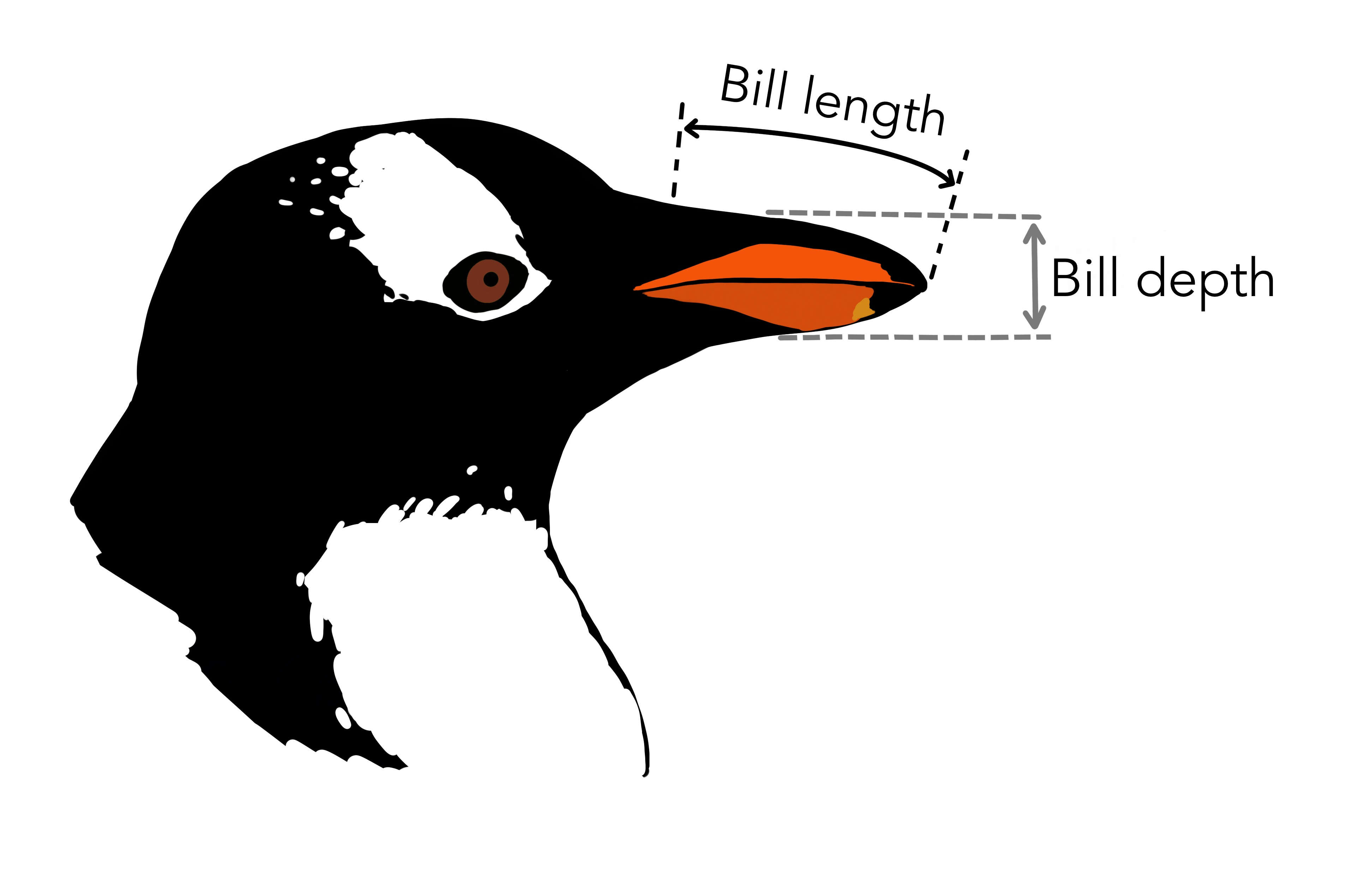
Unser Ziel
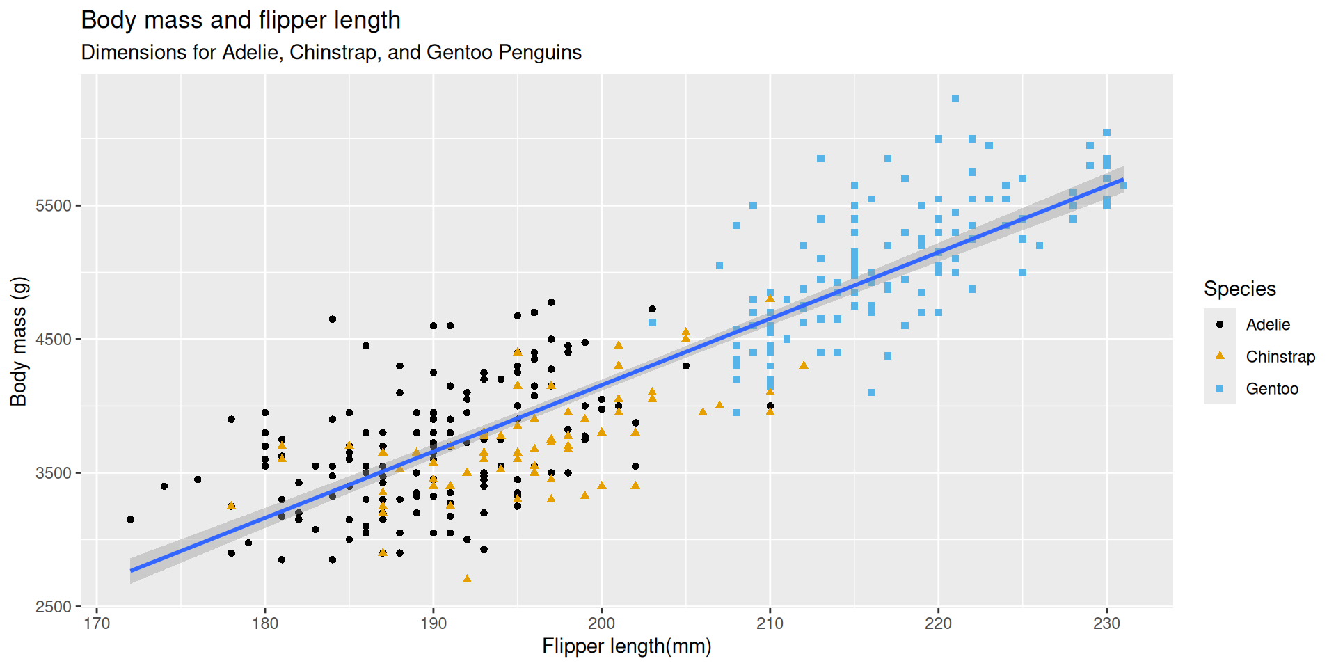
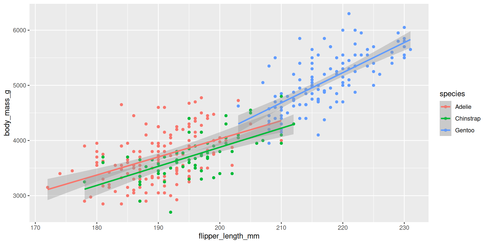
ggplot(
  data = penguins,
  mapping = aes(
    x = flipper_length_mm,
    y = body_mass_g
  )
) +
  geom_point(mapping = aes(colour = species, shape = species)) +
  geom_smooth(method = "lm") +
  labs(
    title = "Body mass and flipper length",
    subtitle = "Dimensions for Adelie, Chinstrap, and Gentoo Penguins",
    x = "Flipper length(mm)",
    y = "Body mass (g)",
    colour = "Species",
    shape = "Species"
  ) +
scale_colour_colorblind()Plot Erstellen

Plot Erstellen
Plot Erstellen
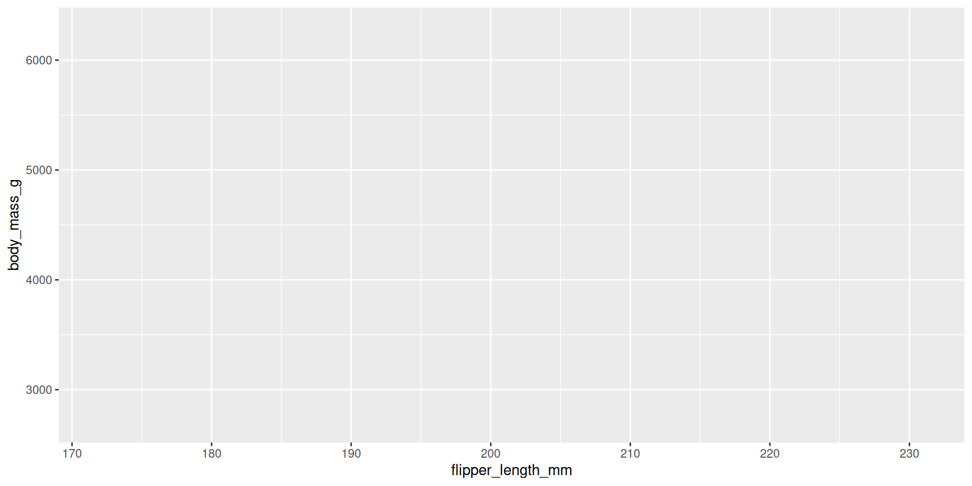
Plot Erstellen
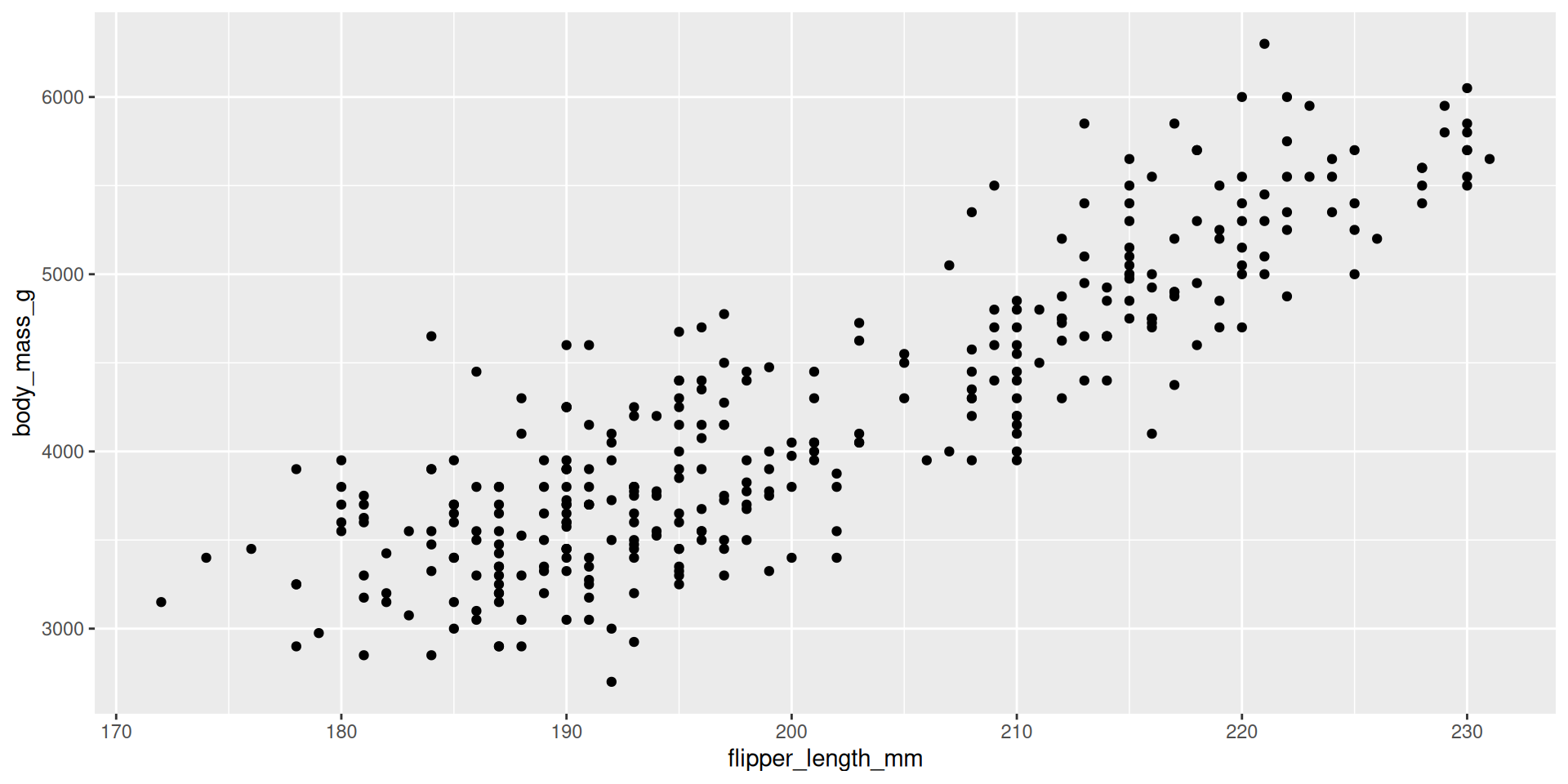
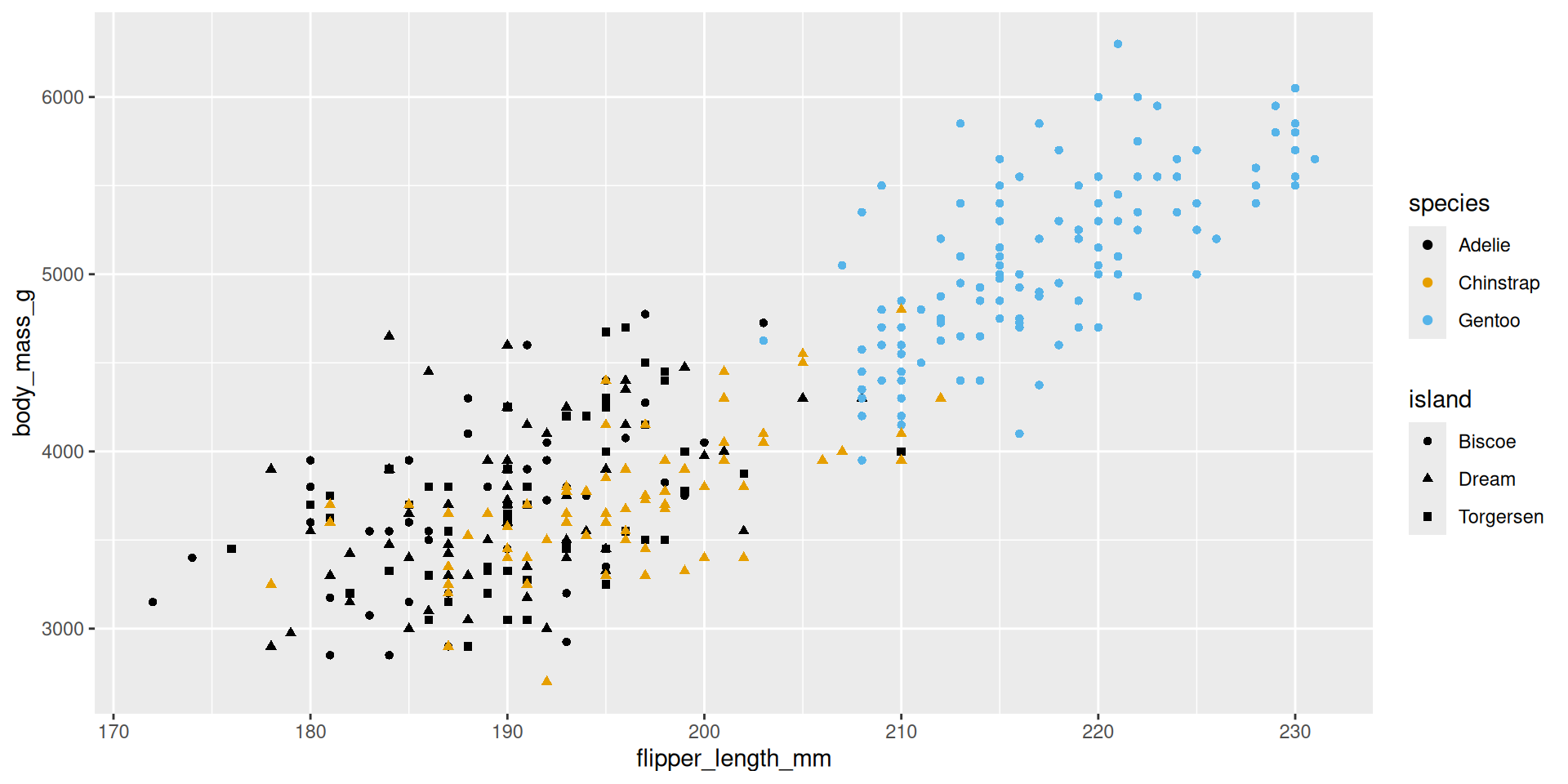
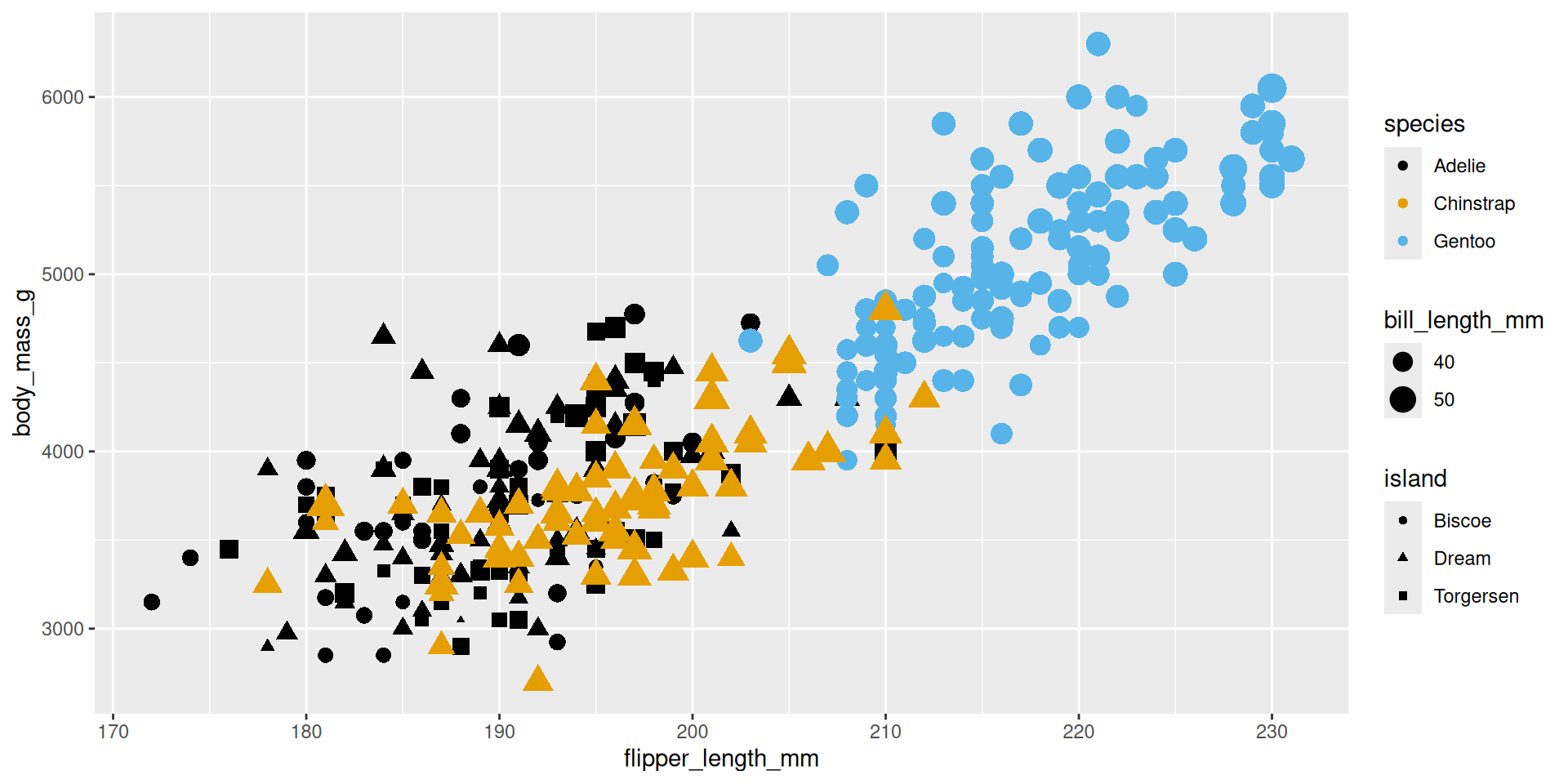
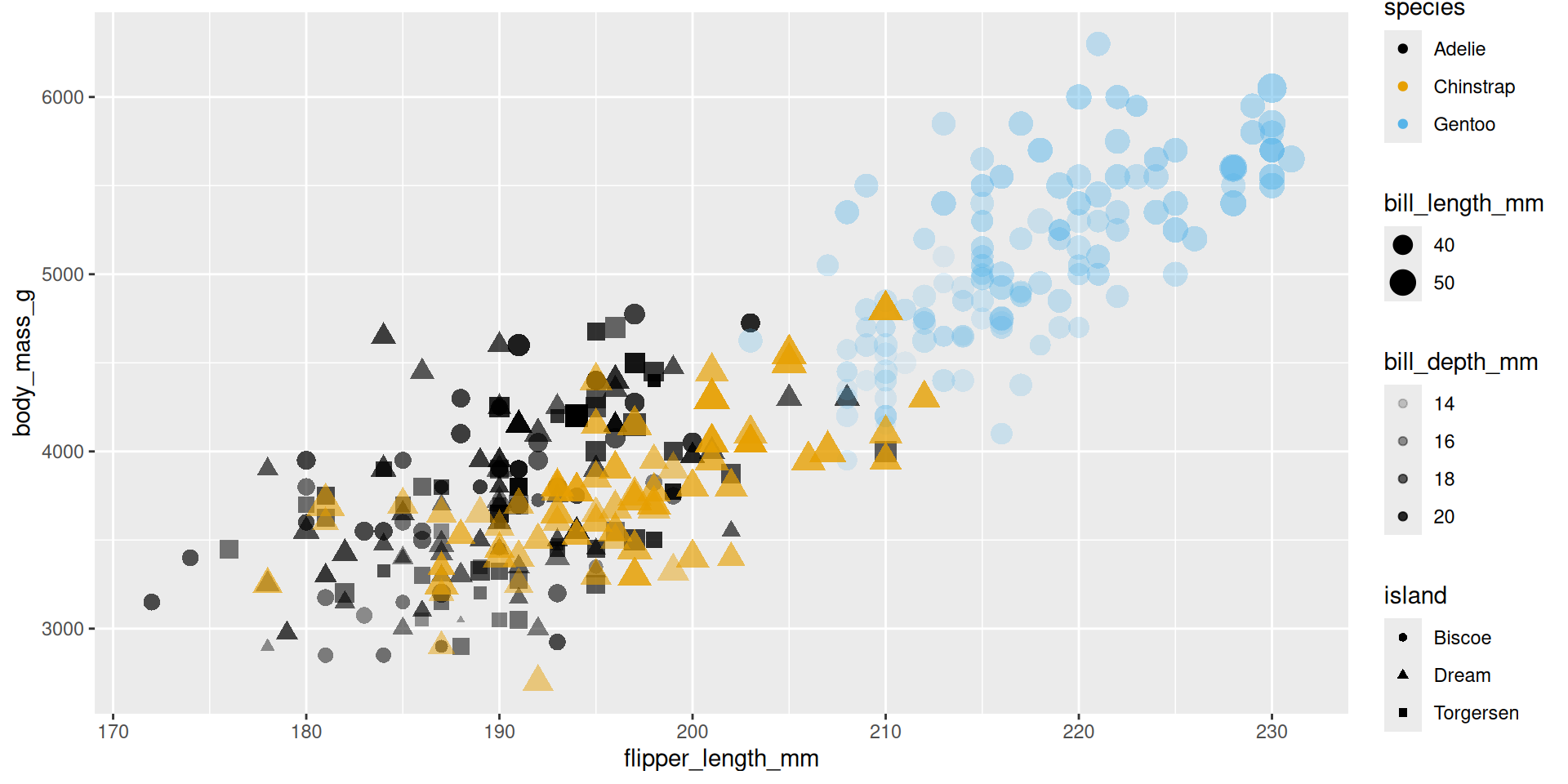
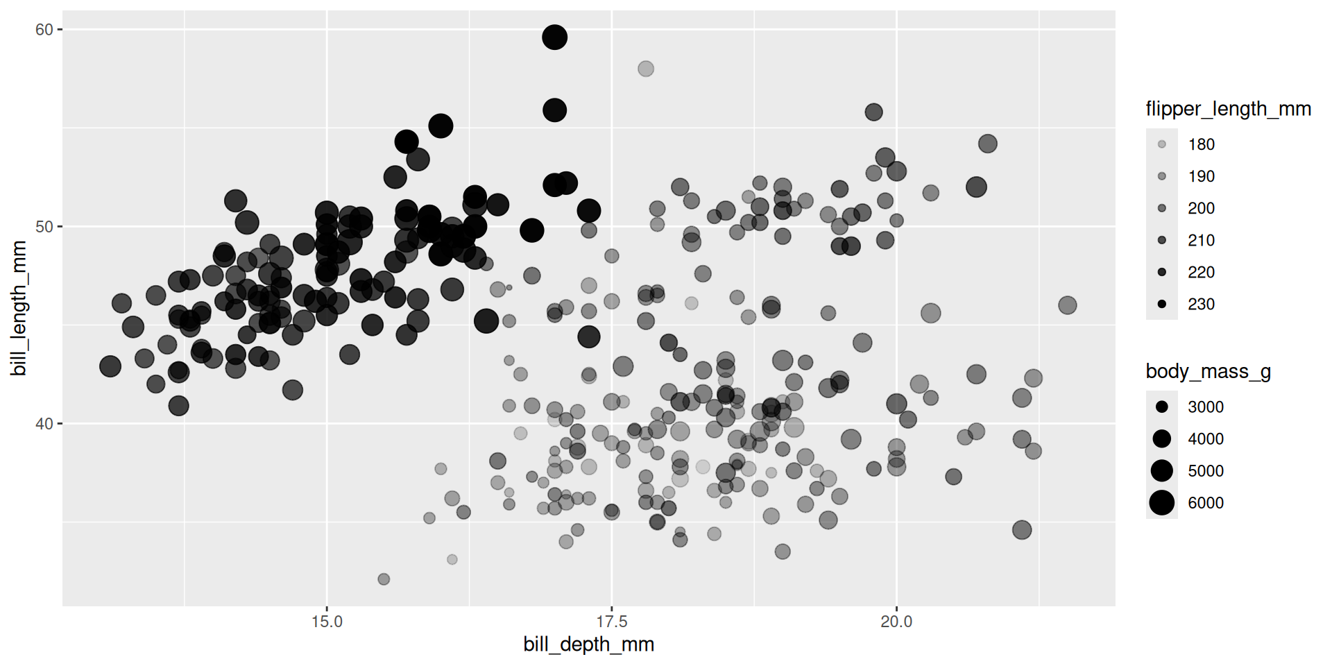
Aesthetics und Schichten
Aesthetics und Schichten
Aesthetics und Schichten
Aesthetics und Schichten
Aesthetics und Schichten
Code
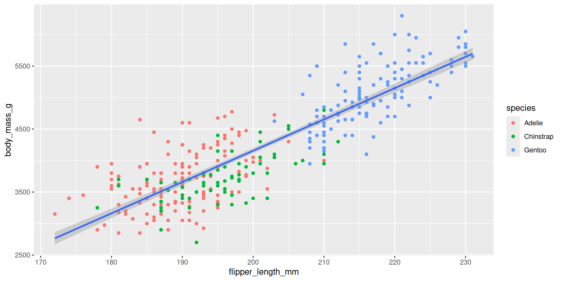
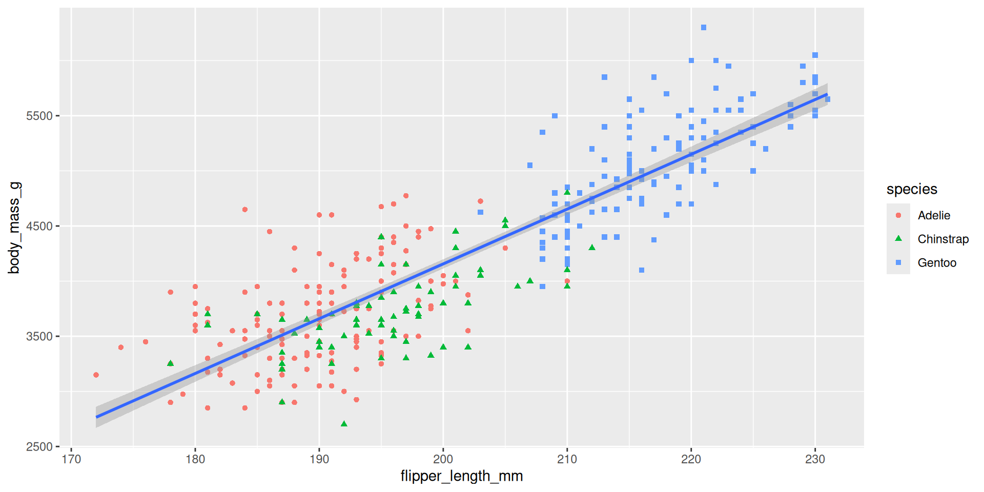
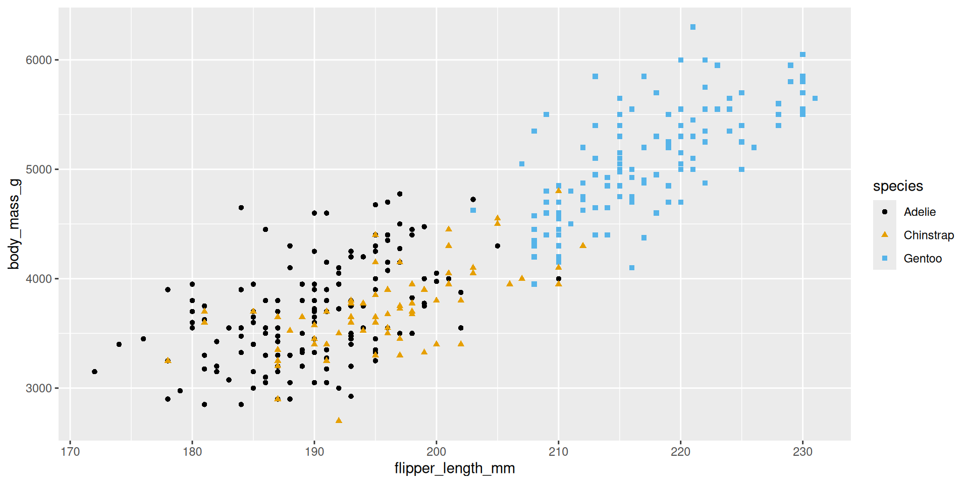
ggplot(
  data = penguins,
  mapping = aes(x = flipper_length_mm, y = body_mass_g)
) +
geom_point(aes(colour = species, shape = species)) +
geom_smooth(method = "lm") +
labs(
title = "Body mass and flipper length",
subtitle = "Dimensions for Adelie, Chinstrap, and Gentoo Penguins",
x = "Flipper length (mm)",
y = "Body mass (g)",
color = "Species",
shape = "Species"
) +
scale_colour_colorblind()
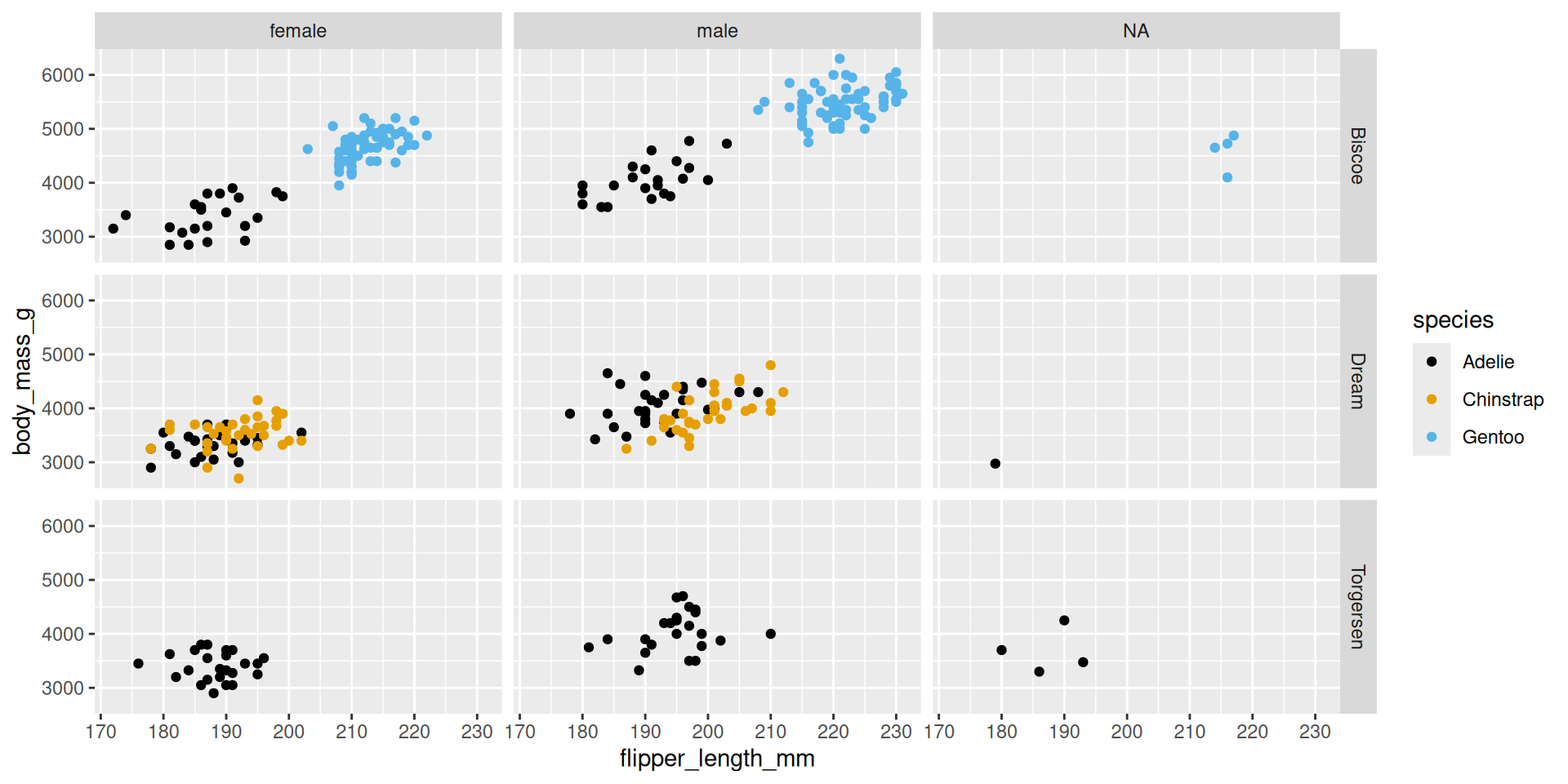
Faceting
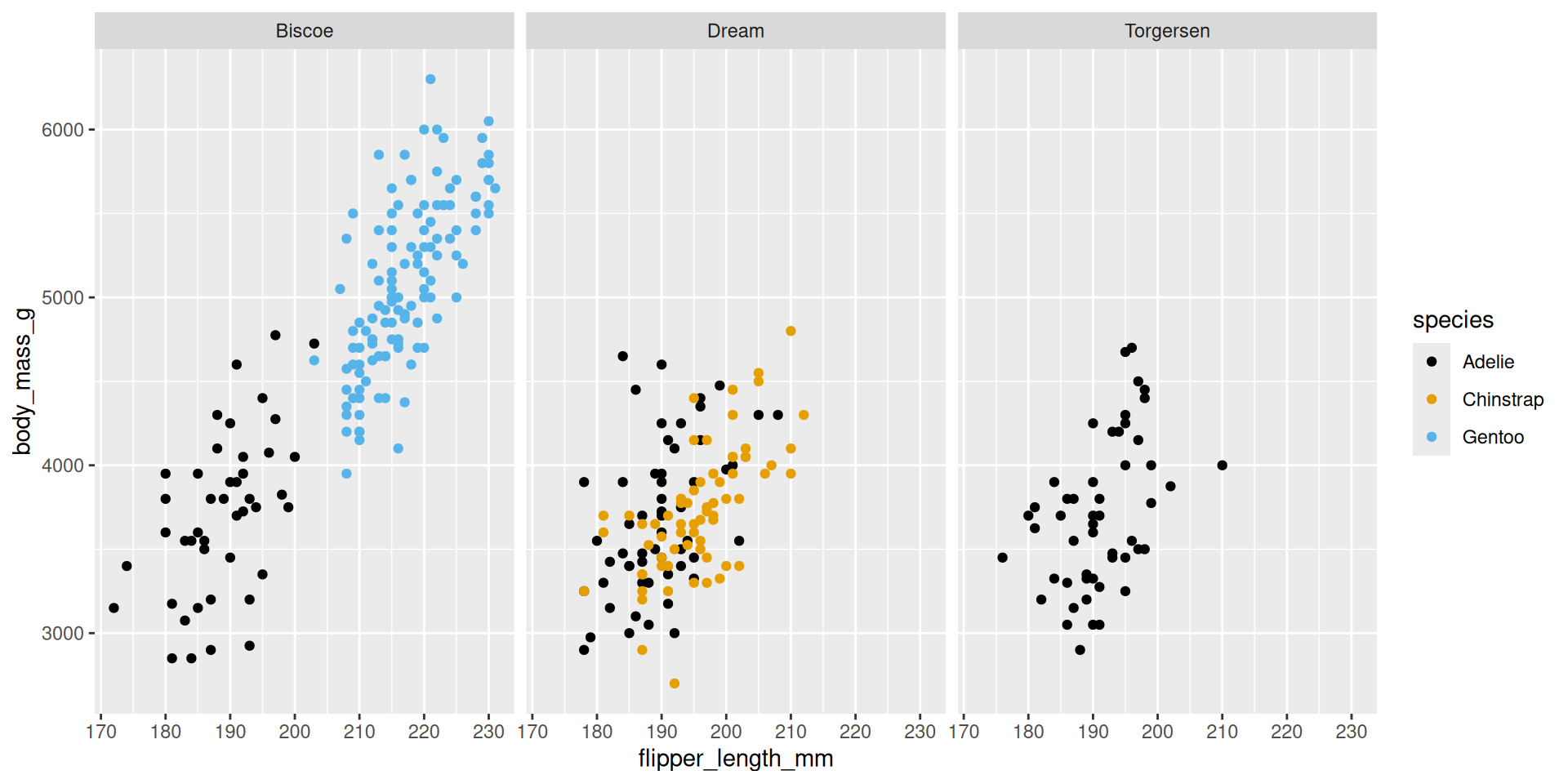
Faceting
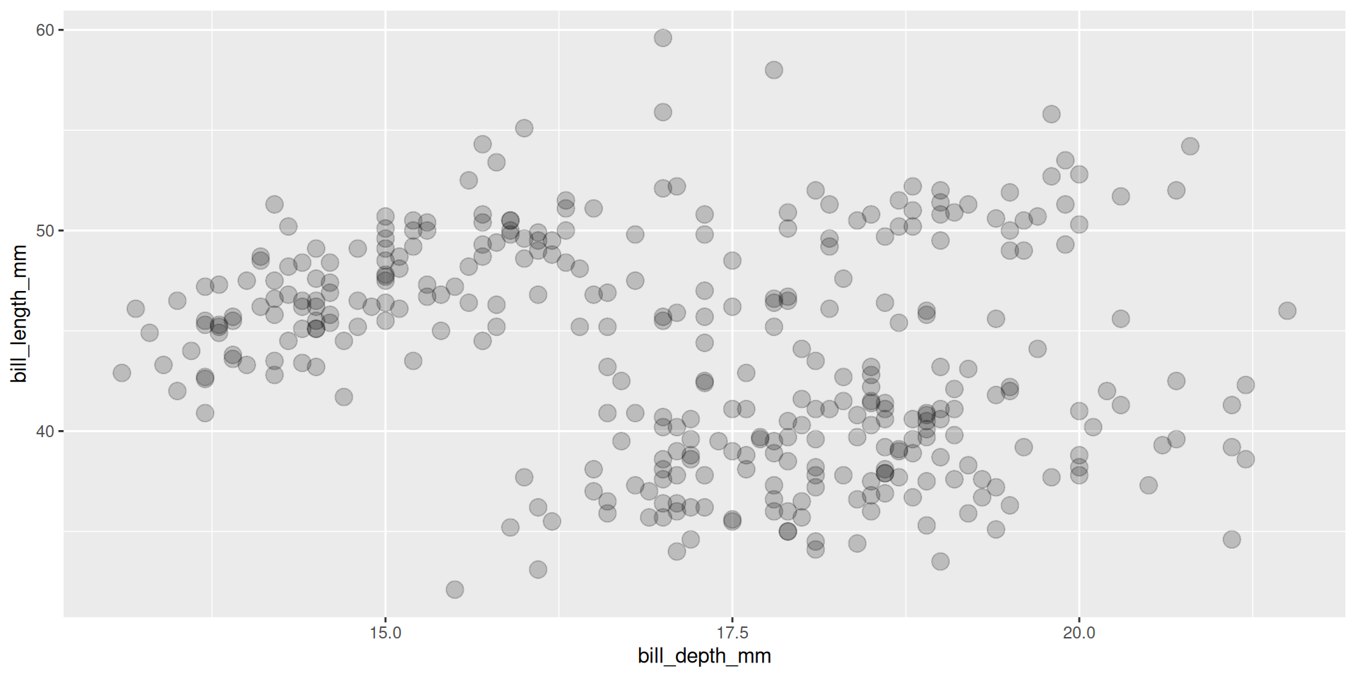
Mapping vs. Setting
R for Data Science
- Das Buch für den Kurs
- Kostenfrei Online
- Tiydverse-Philosophie