Daten importieren, exportieren, zusammenfügen und pivotieren

Unit 4

Ziele für heute

1. grundlegenden Befehle für den Datenimport und -export benennen
2. Befehle zur Zusammenfügung von Daten identifizieren
3. Grundprinzipien des tidy data-Konzepts nennen
4. {tidyr}-Befehle um Daten zu pivotieren auflisten

Daten importieren und exportieren

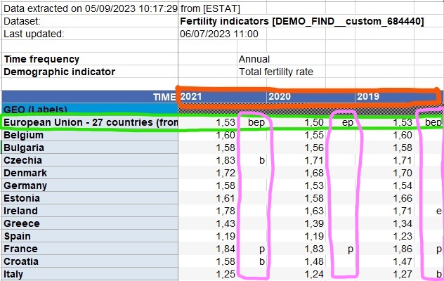
Rechteckige Daten importieren

install.packages("readxl")
library(readxl)

Rechteckige Daten importieren

readr

Funktion	Trennung
read_csv()	,
read_csv2()	;
read_tsv()	⇥ (Tab)
read_delim()	Selbst-definiert

readxl

Funktion	Dateityp
read_excel()	xls oder xlsx

Rechteckige Daten exportieren

install.packages("writexl")
library(writexl)

To export rectangular data, we can use readr and writexl.

Rechteckige Daten exportieren

readr

• write_csv()
• write_csv2()
• write_tsv()
• write_delim()

writexl

• write_xlsx()

Daten lesen

df <- read_delim("data/ogd_10130.csv", delim = ";")
glimpse(df)

Rows: 1,487
Columns: 13
$ date               <date> 2024-11-01, 2024-10-01, 2024-09-01, 2024-08-01, 20…
$ `station/location` <chr> "BAS", "BAS", "BAS", "BAS", "BAS", "BAS", "BAS", "B…
$ station_name       <chr> "Basel / Binningen", "Basel / Binningen", "Basel / …
$ gre000m0           <dbl> 54, 80, 139, 247, 247, 216, 198, 161, 120, 69, 44, …
$ hto000m0           <dbl> 2, 0, 0, 0, 0, 0, 0, 0, 0, 0, 1, 1, 0, 0, 0, 0, 0, …
$ nto000m0           <dbl> 72, 76, 69, 48, 59, 76, 76, 80, 81, 83, 79, 80, 82,…
$ prestam0           <dbl> 984.7, 980.0, 978.5, 979.3, 979.0, 977.6, 976.4, 97…
$ rre150m0           <dbl> 53.5, 81.4, 81.2, 25.8, 62.2, 76.4, 166.7, 39.3, 78…
$ sre000m0           <dbl> 5349, 4917, 7705, 17098, 13519, 9151, 9188, 7279, 6…
$ tre200m0           <dbl> 6.2, 12.9, 15.6, 22.2, 21.0, 18.7, 14.9, 11.1, 9.3,…
$ tre200mn           <dbl> -4.4, 4.8, 3.8, 10.3, 12.6, 8.3, 6.3, 0.4, 1.4, 0.3…
$ tre200mx           <dbl> 16.1, 21.8, 32.1, 35.4, 34.5, 32.2, 27.1, 28.8, 20.…
$ ure200m0           <dbl> 84.3, 85.8, 78.2, 68.7, 70.5, 73.4, 75.0, 68.6, 74.…

Daten schreiben

fussball_weltmeister

# A tibble: 10 × 3
    jahr weltmeisterschaft titeltraeger
   <int> <chr>             <chr>       
 1  2023 Frauen            Spanien     
 2  2022 Männer            Argentinien 
 3  2019 Frauen            USA         
 4  2018 Männer            Frankreich  
 5  2015 Frauen            USA         
 6  2014 Männer            Deutschland 
 7  2011 Frauen            Japan       
 8  2010 Männer            Spanien     
 9  2007 Frauen            Deutschland 
10  2006 Männer            Italien     

write_csv(x = fussball_weltmeister, file = "data/fussball_weltmeister.csv")

Daten wieder einlesen

read_csv("data/fussball_weltmeister.csv")

# A tibble: 10 × 3
    jahr weltmeisterschaft titeltraeger
   <dbl> <chr>             <chr>       
 1  2023 Frauen            Spanien     
 2  2022 Männer            Argentinien 
 3  2019 Frauen            USA         
 4  2018 Männer            Frankreich  
 5  2015 Frauen            USA         
 6  2014 Männer            Deutschland 
 7  2011 Frauen            Japan       
 8  2010 Männer            Spanien     
 9  2007 Frauen            Deutschland 
10  2006 Männer            Italien     

rio

import(), export(), convert()

install.packages("rio")
library(rio)

x <- import("mtcars.csv") 
y <- import("mtcars.rds") # R data format 
z <- import("mtcars.sav") # SPSS
u <- import("mtcars.xlsx")
w <- import("mtcars.json")

export("mtcars.csv")
export(list(mtcars, penguins), "mtcars-penguins.xlsx") # multiple sheets
import("mtcars-penguins.xlsx", which = "penguins") # select one sheet
import_list("mtcars-penguins.xlsx") # import multiple objects

Andere Formate

readRDS() und writeRDS()

• Zwischenergebnisse als CSV zu speichern unzuverlässig, wenn bestimmte Variablentypen beibehalten werden sollen
• read_csv() kann nicht wissen welche Levels eine Faktor-Variable hat
• Alternative: RDS-Dateien, ein R-internes Dateiformat

Store types of columns (factors etc), for use between R scripts. Also binary so take less space.

Variablen-Namen

wetter <- read_delim("data/ogd_12030.csv")
names(wetter)

 [1] "Datum"                       "Jahr"                       
 [3] "Globalstrahlung in W/m2"     "Gesamtschneemenge"          
 [5] "Gesamtbewölkung"             "Luftdruck in hPa"           
 [7] "Niederschlag"                "Sonnenscheindauer"          
 [9] "Tagesmittel Lufttemperatur"  "Tagesminimum Lufttemperatur"
[11] "Tagesmaximum Lufttemperatur" "Relative Luftfeuchtigkeit"  

wetter |> 
  filter(Globalstrahlung in W/m2 > 111)

Error in parse(text = input): <text>:2:26: unexpected 'in'
1: wetter |> 
2:   filter(Globalstrahlung in
                            ^

Variablen-Namen - Backticks `

wetter |> 
  filter(`Globalstrahlung in W/m2` > 111)

# A tibble: 8,013 × 12
   Datum       Jahr `Globalstrahlung in W/m2` Gesamtschneemenge Gesamtbewölkung
   <date>     <dbl>                     <dbl>             <dbl>           <dbl>
 1 2001-02-15  2001                       113                 0              17
 2 2001-02-19  2001                       117                 0              42
 3 2001-02-26  2001                       113                 0              13
 4 2001-02-27  2001                       118                 0              88
 5 2001-03-24  2001                       122                 0              88
 6 2001-03-25  2001                       112                 0              92
 7 2001-04-02  2001                       218                 0              83
 8 2001-04-05  2001                       188                 0              50
 9 2001-04-13  2001                       203                 0              63
10 2001-04-14  2001                       160                 0              79
# ℹ 8,003 more rows
# ℹ 7 more variables: `Luftdruck in hPa` <dbl>, Niederschlag <dbl>,
#   Sonnenscheindauer <dbl>, `Tagesmittel Lufttemperatur` <dbl>,
#   `Tagesminimum Lufttemperatur` <dbl>, `Tagesmaximum Lufttemperatur` <dbl>,
#   `Relative Luftfeuchtigkeit` <dbl>

Mühsam

Variablen-Namen - {readr}-Funktion

wetter<- read_delim(
  "data/ogd_12030.csv",
  col_names = c(
    "datum",
    "jahr",
    "globalstrahlung_in_w_m2",
    "gesamtschneemenge",
    "gesamtbewolkung",
    "luftdruck_in_h_pa",
    "niederschlag",
    "sonnenscheindauer",
    "tagesmittel_lufttemperatur",
    "tagesminimum_lufttemperatur",
    "tagesmaximum_lufttemperatur",
    "relative_luftfeuchtigkeit"
  )
)
names(wetter)

 [1] "datum"                       "jahr"                       
 [3] "globalstrahlung_in_w_m2"     "gesamtschneemenge"          
 [5] "gesamtbewolkung"             "luftdruck_in_h_pa"          
 [7] "niederschlag"                "sonnenscheindauer"          
 [9] "tagesmittel_lufttemperatur"  "tagesminimum_lufttemperatur"
[11] "tagesmaximum_lufttemperatur" "relative_luftfeuchtigkeit"  

Auch mühsam

Variablen-Namen - {janitor}

# install.packages("janitor")
library(janitor)

wetter <- read_delim("data/ogd_12030.csv")

wetter |> 
  clean_names() |> 
  names()

 [1] "datum"                       "jahr"                       
 [3] "globalstrahlung_in_w_m2"     "gesamtschneemenge"          
 [5] "gesamtbewolkung"             "luftdruck_in_h_pa"          
 [7] "niederschlag"                "sonnenscheindauer"          
 [9] "tagesmittel_lufttemperatur"  "tagesminimum_lufttemperatur"
[11] "tagesmaximum_lufttemperatur" "relative_luftfeuchtigkeit"  

Praktikum 04a: Daten importieren und exportieren

prak-04a-import-export.qmd

30:00

Break ☕ 🍵 🍜

10:00

Daten-Transformation mit dplyr

Zeilen: auswählen, anordnen

Spalten: aswählen, anordnen, umbenennen, erstellen

Gruppen: zusammenfassen, zählen

Tabellen: zusammenfügen

Daten zusammenfügen mit dplyr

Wir…

haben mehrere Dataframes

wollen diese zusammenbringen

Daten: Frauen in der Wissenschaft

Informationen zu 10 Frauen in der Wissenschaft welche die Welt verändert haben.

Quelle: Discover Magazine

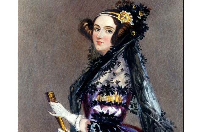
Inputs: drei Dataframes

• professions
• dates
• works

name	profession
Ada Lovelace	Mathematician
Marie Curie	Physicist and Chemist
Janaki Ammal	Botanist
Chien-Shiung Wu	Physicist
Katherine Johnson	Mathematician
Rosalind Franklin	Chemist
Vera Rubin	Astronomer
Gladys West	Mathematician
Flossie Wong-Staal	Virologist and Molecular Biologist
Jennifer Doudna	Biochemist

name	birth_year	death_year
Janaki Ammal	1897	1984
Chien-Shiung Wu	1912	1997
Katherine Johnson	1918	2020
Rosalind Franklin	1920	1958
Vera Rubin	1928	2016
Gladys West	1930	NA
Flossie Wong-Staal	1947	NA
Jennifer Doudna	1964	NA

name	known_for
Ada Lovelace	first computer algorithm
Marie Curie	theory of radioactivity, discovery of elements polonium and radium, first woman to win a Nobel Prize
Janaki Ammal	hybrid species, biodiversity protection
Chien-Shiung Wu	confim and refine theory of radioactive beta decy, Wu experiment overturning theory of parity
Katherine Johnson	calculations of orbital mechanics critical to sending the first Americans into space
Vera Rubin	existence of dark matter
Gladys West	mathematical modeling of the shape of the Earth which served as the foundation of GPS technology
Flossie Wong-Staal	first scientist to clone HIV and create a map of its genes which led to a test for the virus
Jennifer Doudna	one of the primary developers of CRISPR, a ground-breaking technology for editing genomes

Gewünschter Output

name	profession	birth_year	death_year	known_for
Ada Lovelace	Mathematician	NA	NA	first computer algorithm
Marie Curie	Physicist and Chemist	NA	NA	theory of radioactivity, discovery of elements polonium and radium, first woman to win a Nobel Prize
Janaki Ammal	Botanist	1897	1984	hybrid species, biodiversity protection
Chien-Shiung Wu	Physicist	1912	1997	confim and refine theory of radioactive beta decy, Wu experiment overturning theory of parity
Katherine Johnson	Mathematician	1918	2020	calculations of orbital mechanics critical to sending the first Americans into space
Rosalind Franklin	Chemist	1920	1958	NA
Vera Rubin	Astronomer	1928	2016	existence of dark matter
Gladys West	Mathematician	1930	NA	mathematical modeling of the shape of the Earth which served as the foundation of GPS technology
Flossie Wong-Staal	Virologist and Molecular Biologist	1947	NA	first scientist to clone HIV and create a map of its genes which led to a test for the virus
Jennifer Doudna	Biochemist	1964	NA	one of the primary developers of CRISPR, a ground-breaking technology for editing genomes

Hier sehen wir unseren gewünschten Output. Das Ziel nachdem die drei Dataframes zusammengefügt wurden:

• name und profession aus dem ersten Dataframe
• name, birth_year und death_year aus dem zweiten Dataframe
• name und known_for aus dem dritten Dataframe

Inputs: drei Dataframes

names(professions)

[1] "name"       "profession"

names(dates)

[1] "name"       "birth_year" "death_year"

names(works)

[1] "name"      "known_for"

nrow(professions)

[1] 10

nrow(dates)

[1] 8

nrow(works)

[1] 9

• Name ist hier sozusagen der Schlüssel
• Professions hat die komplette Info während bei den anderen etwas fehlt

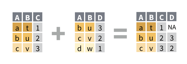
Dataframes zusammenfügen

***_join(x, y)

• left_join(x, y): alle Reihen aus x
• right_join(x, y): alle Reihen aus y
• full_join(x, y): alle Reihen aus x und y
• inner_join(x, y): gemeinsame Reihen aus x und y
• semi_join(x, y): wie inner_join(x, y), nur Spalten aus x
• anti_join(x, y): Reihen aus x ohne Übereinstimmung in y

Beispiel

Für die nächsten Folien

x

# A tibble: 3 × 2
     id var_x
  <dbl> <chr>
1     1 x1   
2     2 x2   
3     3 x3   

y

# A tibble: 3 × 2
     id var_y
  <dbl> <chr>
1     1 y1   
2     2 y2   
3     4 y4   

left_join()

left_join(x, y)

# A tibble: 3 × 3
     id var_x var_y
  <dbl> <chr> <chr>
1     1 x1    y1   
2     2 x2    y2   
3     3 x3    <NA> 

left_join()

professions |>
  left_join(dates)

# A tibble: 10 × 4
   name               profession                         birth_year death_year
   <chr>              <chr>                                   <dbl>      <dbl>
 1 Ada Lovelace       Mathematician                              NA         NA
 2 Marie Curie        Physicist and Chemist                      NA         NA
 3 Janaki Ammal       Botanist                                 1897       1984
 4 Chien-Shiung Wu    Physicist                                1912       1997
 5 Katherine Johnson  Mathematician                            1918       2020
 6 Rosalind Franklin  Chemist                                  1920       1958
 7 Vera Rubin         Astronomer                               1928       2016
 8 Gladys West        Mathematician                            1930         NA
 9 Flossie Wong-Staal Virologist and Molecular Biologist       1947         NA
10 Jennifer Doudna    Biochemist                               1964         NA

right_join()

right_join(x, y)

# A tibble: 3 × 3
     id var_x var_y
  <dbl> <chr> <chr>
1     1 x1    y1   
2     2 x2    y2   
3     4 <NA>  y4   

right_join

professions |>
  right_join(dates)

# A tibble: 8 × 4
  name               profession                         birth_year death_year
  <chr>              <chr>                                   <dbl>      <dbl>
1 Janaki Ammal       Botanist                                 1897       1984
2 Chien-Shiung Wu    Physicist                                1912       1997
3 Katherine Johnson  Mathematician                            1918       2020
4 Rosalind Franklin  Chemist                                  1920       1958
5 Vera Rubin         Astronomer                               1928       2016
6 Gladys West        Mathematician                            1930         NA
7 Flossie Wong-Staal Virologist and Molecular Biologist       1947         NA
8 Jennifer Doudna    Biochemist                               1964         NA

full_join()

full_join(x, y)

# A tibble: 4 × 3
     id var_x var_y
  <dbl> <chr> <chr>
1     1 x1    y1   
2     2 x2    y2   
3     3 x3    <NA> 
4     4 <NA>  y4   

full_join()

dates |>
  full_join(works)

# A tibble: 10 × 4
   name               birth_year death_year known_for                           
   <chr>                   <dbl>      <dbl> <chr>                               
 1 Janaki Ammal             1897       1984 hybrid species, biodiversity protec…
 2 Chien-Shiung Wu          1912       1997 confim and refine theory of radioac…
 3 Katherine Johnson        1918       2020 calculations of orbital mechanics c…
 4 Rosalind Franklin        1920       1958 <NA>                                
 5 Vera Rubin               1928       2016 existence of dark matter            
 6 Gladys West              1930         NA mathematical modeling of the shape …
 7 Flossie Wong-Staal       1947         NA first scientist to clone HIV and cr…
 8 Jennifer Doudna          1964         NA one of the primary developers of CR…
 9 Ada Lovelace               NA         NA first computer algorithm            
10 Marie Curie                NA         NA theory of radioactivity,  discovery…

Alles in einer Code-Sequenz

professions |>
  left_join(dates) |>
  left_join(works)

# A tibble: 10 × 5
   name               profession                 birth_year death_year known_for
   <chr>              <chr>                           <dbl>      <dbl> <chr>    
 1 Ada Lovelace       Mathematician                      NA         NA first co…
 2 Marie Curie        Physicist and Chemist              NA         NA theory o…
 3 Janaki Ammal       Botanist                         1897       1984 hybrid s…
 4 Chien-Shiung Wu    Physicist                        1912       1997 confim a…
 5 Katherine Johnson  Mathematician                    1918       2020 calculat…
 6 Rosalind Franklin  Chemist                          1920       1958 <NA>     
 7 Vera Rubin         Astronomer                       1928       2016 existenc…
 8 Gladys West        Mathematician                    1930         NA mathemat…
 9 Flossie Wong-Staal Virologist and Molecular …       1947         NA first sc…
10 Jennifer Doudna    Biochemist                       1964         NA one of t…

join_by()

mitarbeiter <- tibble(
  id = c(1, 2, 3),
  name = c("Alice", "Bob", "Charlie")
)
mitarbeiter

# A tibble: 3 × 2
     id name   
  <dbl> <chr>  
1     1 Alice  
2     2 Bob    
3     3 Charlie

gehälter <- tibble(
  persid = c(1, 2, 4),
  gehalt = c(50000, 60000, 70000)
)
gehälter

# A tibble: 3 × 2
  persid gehalt
   <dbl>  <dbl>
1      1  50000
2      2  60000
3      4  70000

join_by()

ergebnis <- mitarbeiter |>
  left_join(gehälter, join_by(id == persid))
ergebnis

# A tibble: 3 × 3
     id name    gehalt
  <dbl> <chr>    <dbl>
1     1 Alice    50000
2     2 Bob      60000
3     3 Charlie     NA

Praktikum 04b: Daten zusammenfügen

prak-04b-join-firmen.qmd

20:00

Break ☕ 🍵 🍜

10:00

Tidy Data

Tidy Data

“Alle glücklichen Familien gleichen einander, jede unglückliche Familie ist auf ihre eigene Weise unglücklich.” – Leo Tolstoy

“Tidy datasets are all alike, but every messy dataset is messy in its own way.” –– Hadley Wickham

tidy = ordentlich, sauber, aufgeräumt.

“Happy families are all alike; every unhappy family is unhappy in its own way.” – Leo Tolstoy

Tidy Data

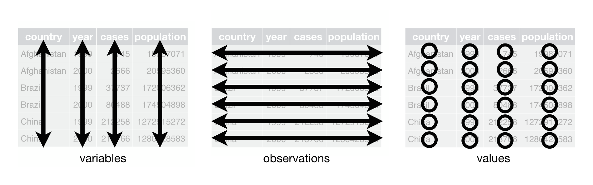
1. Jede Variable muss eine eigene Spalte haben
2. Jede Beobachtung muss eine eigene Zeile haben
3. Jeder Wert muss eine eigene Zelle haben

1. Each variable must have its own column.
2. Each observation must have its own row.
3. Each value must have its own cell.

❓

species	island	bill_length_mm	bill_depth_mm	flipper_length_mm	body_mass_g	sex	year
Adelie	Torgersen	39.1	18.7	181	3750	male	2007
Adelie	Torgersen	39.5	17.4	186	3800	female	2007
Adelie	Torgersen	40.3	18.0	195	3250	female	2007
Adelie	Torgersen	NA	NA	NA	NA	NA	2007
Adelie	Torgersen	36.7	19.3	193	3450	female	2007
Adelie	Torgersen	39.3	20.6	190	3650	male	2007
Adelie	Torgersen	38.9	17.8	181	3625	female	2007
Adelie	Torgersen	39.2	19.6	195	4675	male	2007
Adelie	Torgersen	34.1	18.1	193	3475	NA	2007
Adelie	Torgersen	42.0	20.2	190	4250	NA	2007
Adelie	Torgersen	37.8	17.1	186	3300	NA	2007
Adelie	Torgersen	37.8	17.3	180	3700	NA	2007
Adelie	Torgersen	41.1	17.6	182	3200	female	2007
Adelie	Torgersen	38.6	21.2	191	3800	male	2007

❓

Quelle: Bundesamt für Statistik - Ständige Wohnbevölkerung nach Altersklasse und Altersmasszahlen nach Kanton, Provisorische Jahresergebnisse, 2020

❓

Quelle: Bundesamt für Statistik - Ständige Wohnbevölkerung nach Altersklasse und Altersmasszahlen nach Kanton, Provisorische Jahresergebnisse, 2020

❓

Quelle: Bundesamt für Statistik - Ständige Wohnbevölkerung nach Altersklasse und Altersmasszahlen nach Kanton, Provisorische Jahresergebnisse, 2020

❓

Quelle: Eurostat Fertility Indicators

❓

Variable Jahr als Zeile

Quelle: Eurostat Fertility Indicators

❓

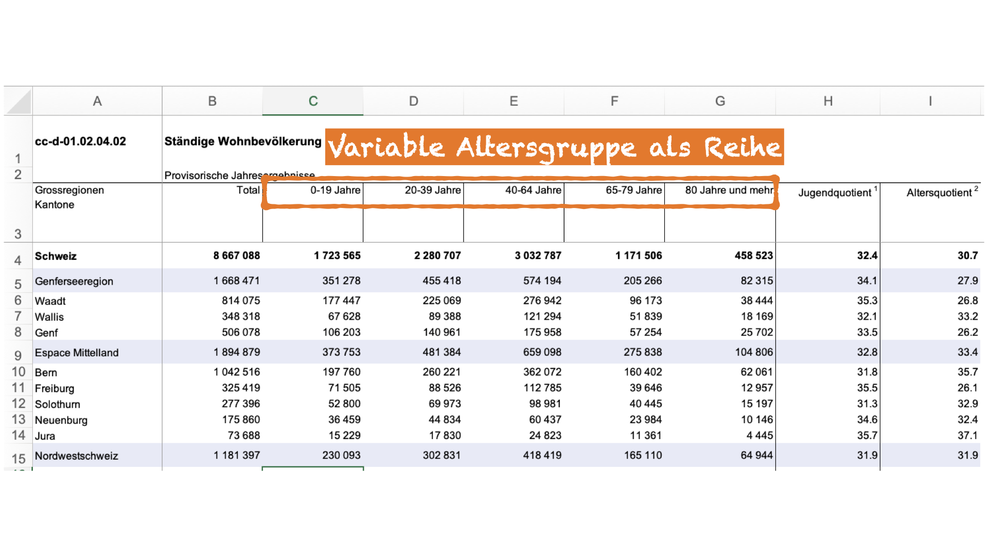
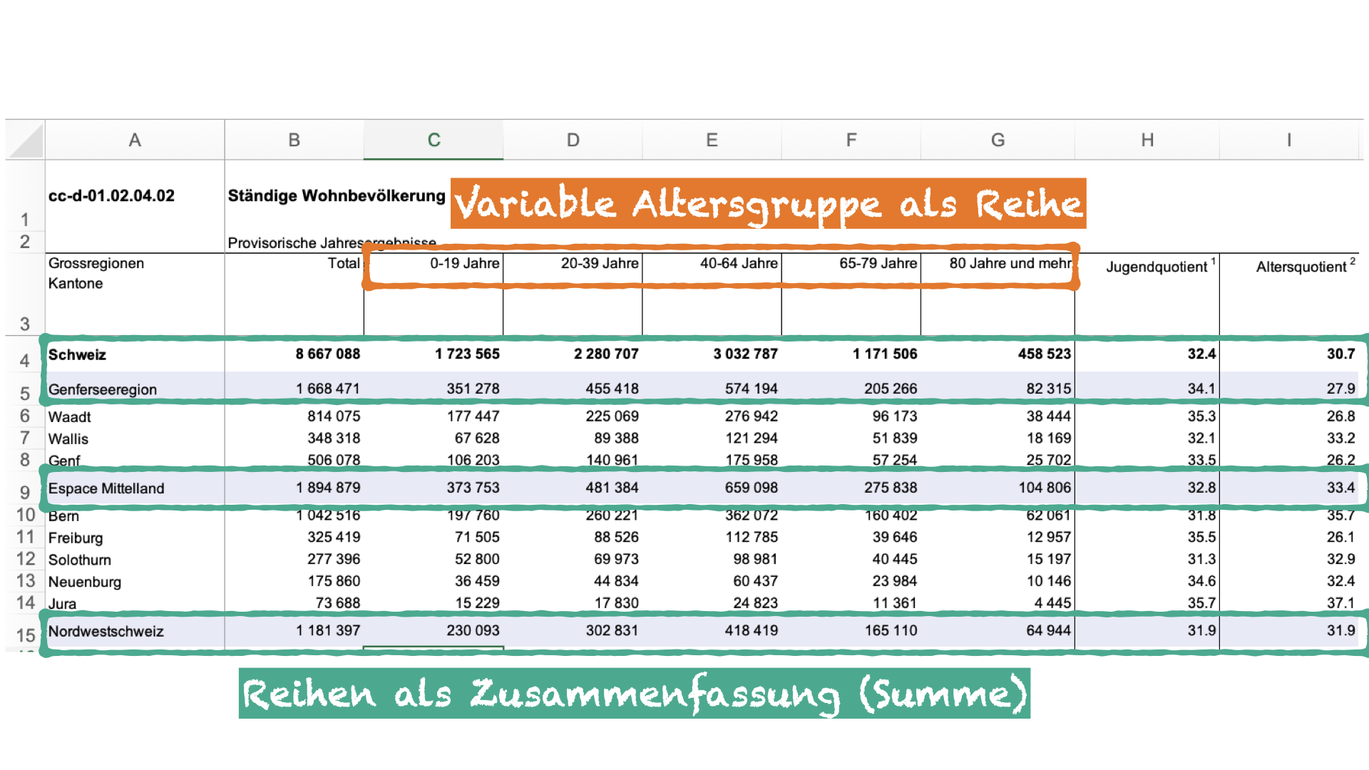
Variable Jahr als Zeile

Zeile als Zusammenfassung (Durchschnitt)

Quelle: Eurostat Fertility Indicators

❓

Variable Jahr als Zeile

Zeile als Zusammenfassung (Durchschnitt)

3 Spalten für eine Variable

Für Darstellungszwecke ist das ok, tatsächlich nützlich. Aber wenn wir mit Rohdaten arbeiten wollen, dann sollten diese Tidy sein.

• Title block
• TIME should be “GEO Label” for the column underneath it
• Years should be converted into a single column “Year” and the value should say “fertility rate”. What if we wanted to add data for population, number of women, or any other value for that year?
• bep, b etc are codes for how the data was collected. It should all be in one column
• : stands for NA, so convert

Quelle: Eurostat Fertility Indicators

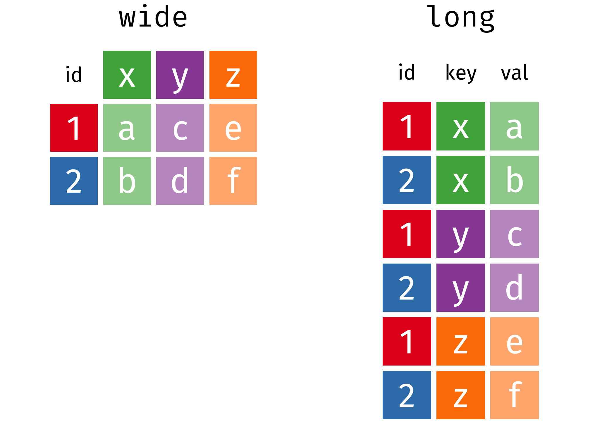
Daten mit tidyr aufräumen

• Daten umformen/pivotieren (erweitern, verlängern)

• Zellen teilen
• Fehlende Werte (NA) behandeln

Erinnernt euch an das Konzept der tidy data? Jede Spalte ist eine Variable, jede Zeile ist eine Beobachtung, jede Zelle ist ein Wert. Die Tidyverse-Funktionen erwarten Tidy-Daten. So oft müssen wir die Daten umformen, indem wir Zeilen und Spalten drehen und Zellen teilen, um neue Variablen oder Beobachtungen zu erstellen. Diese Aufräumfunktionen werden durch das Paket Tidyr gewährleistet. Darüber hinaus bietet Tidyr Tools zum Umgang mit fehlenden Daten.

Daten pivotieren

Nicht das…

sondern das!

Daten pivotieren

wide |>
  pivot_longer(
    cols = x:z,
    names_to = "key",
    values_to = "val"
  )

long |>
  pivot_wider(
    names_from = key,
    values_from = val
  )

country	year	cases	population
Afghanistan	1999	745	19987071
Afghanistan	2000	2666	20595360
Brazil	1999	37737	172006362
Brazil	2000	80488	174504898
China	1999	212258	1272915272
China	2000	213766	1280428583

country	type	1999	2000
Afghanistan	cases	745	2666
Afghanistan	population	19987071	20595360
Brazil	cases	37737	80488
Brazil	population	172006362	174504898
China	cases	212258	213766
China	population	1272915272	1280428583

country	year	type	count
Afghanistan	1999	cases	745
Afghanistan	1999	population	19987071
Afghanistan	2000	cases	2666
Afghanistan	2000	population	20595360
Brazil	1999	cases	37737
Brazil	1999	population	172006362
Brazil	2000	cases	80488
Brazil	2000	population	174504898
China	1999	cases	212258
China	1999	population	1272915272
China	2000	cases	213766
China	2000	population	1280428583

country	year	rate
Afghanistan	1999	745/19987071
Afghanistan	2000	2666/20595360
Brazil	1999	37737/172006362
Brazil	2000	80488/174504898
China	1999	212258/1272915272
China	2000	213766/1280428583

In diesem Beispiel werden dieselben Daten auf vier verschiedene Arten organisiert. Jeder Datensatz zeigt die gleichen Werte von vier Variablen: Land, Jahr, Bevölkerung und Anzahl der dokumentierten Fälle von TB (Tuberkulose), aber jeder Datensatz organisiert die Werte auf unterschiedliche Weise.

Dies sind alles Darstellungen derselben Daten, die jedoch nicht gleichermaßen einfach zu verwenden sind.

Mit welcher Tabelle ist es im Tidyverse viel einfacher zu arbeiten?

Tabelle 1, da sie tidy ist.

country	year	cases	population
Afghanistan	1999	745	19987071
Afghanistan	2000	2666	20595360
Brazil	1999	37737	172006362
Brazil	2000	80488	174504898
China	1999	212258	1272915272
China	2000	213766	1280428583

table1 |>
  mutate(rate = cases / population * 10000)

# A tibble: 6 × 5
  country      year  cases population  rate
  <chr>       <dbl>  <dbl>      <dbl> <dbl>
1 Afghanistan  1999    745   19987071 0.373
2 Afghanistan  2000   2666   20595360 1.29 
3 Brazil       1999  37737  172006362 2.19 
4 Brazil       2000  80488  174504898 4.61 
5 China        1999 212258 1272915272 1.67 
6 China        2000 213766 1280428583 1.67 

Wenn wir die Tuberkuloserate für jedes Land pro 10,000 Einwohner berechnen möchten, dividieren wir einfach die Spalte cases durch die Spalte population und multiplizieren mit 10,000.

country	year	type	count
Afghanistan	1999	cases	745
Afghanistan	1999	population	19987071
Afghanistan	2000	cases	2666
Afghanistan	2000	population	20595360
Brazil	1999	cases	37737
Brazil	1999	population	172006362
Brazil	2000	cases	80488
Brazil	2000	population	174504898
China	1999	cases	212258
China	1999	population	1272915272
China	2000	cases	213766
China	2000	population	1280428583

table2 |>
  pivot_wider(
    names_from = type,
    values_from = count
  ) |>
  mutate(rate = cases / population * 10000)

# A tibble: 6 × 5
  country      year  cases population  rate
  <chr>       <dbl>  <dbl>      <dbl> <dbl>
1 Afghanistan  1999    745   19987071 0.373
2 Afghanistan  2000   2666   20595360 1.29 
3 Brazil       1999  37737  172006362 2.19 
4 Brazil       2000  80488  174504898 4.61 
5 China        1999 212258 1272915272 1.67 
6 China        2000 213766 1280428583 1.67 

Allerdings ist es mit der zweiten Tabelle nicht so einfach. Um die Rate zu berechnen, müssen wir zunächst die Daten erweitern, um zwei neue Variablen zu erstellen, deren Namen vom type Variable abgeleitet sind.

country	year	rate
Afghanistan	1999	745/19987071
Afghanistan	2000	2666/20595360
Brazil	1999	37737/172006362
Brazil	2000	80488/174504898
China	1999	212258/1272915272
China	2000	213766/1280428583

table3 |>
  separate_wider_delim(
    cols = rate,
    delim = "/",
    names = c("cases", "population")
  ) |>
  mutate(
    # separate_wider_delim() outputs character
    cases = as.numeric(cases),
    population = as.numeric(population),
    rate = cases / population * 10000
  )

# A tibble: 6 × 5
  country      year  cases population  rate
  <chr>       <dbl>  <dbl>      <dbl> <dbl>
1 Afghanistan  1999    745   19987071 0.373
2 Afghanistan  2000   2666   20595360 1.29 
3 Brazil       1999  37737  172006362 2.19 
4 Brazil       2000  80488  174504898 4.61 
5 China        1999 212258 1272915272 1.67 
6 China        2000 213766 1280428583 1.67 

Die dritte Tabelle erfordert einen anderen Ansatz. Wir müssen die rate Spalte in zwei Spalten aufteilen. Auch hier kommt mit Tidyr Abhilfe mit der Funktion separate_wider_delim().

Beachtet, dass die Ausgabespalten den Datentyp character haben. Wir setzen ihren Typ auf numeric um, damit wir numerische Operationen ausführen können. Mehr dazu im nächsten Abschnitt.

country	type	1999	2000
Afghanistan	cases	745	2666
Afghanistan	population	19987071	20595360
Brazil	cases	37737	80488
Brazil	population	172006362	174504898
China	cases	212258	213766
China	population	1272915272	1280428583

❓

table4 |> 
  pivot_longer(cols = `1999`:`2000`, names_to = "year")

# A tibble: 12 × 4
   country     type       year       value
   <chr>       <chr>      <chr>      <dbl>
 1 Afghanistan cases      1999         745
 2 Afghanistan cases      2000        2666
 3 Afghanistan population 1999    19987071
 4 Afghanistan population 2000    20595360
 5 Brazil      cases      1999       37737
 6 Brazil      cases      2000       80488
 7 Brazil      population 1999   172006362
 8 Brazil      population 2000   174504898
 9 China       cases      1999      212258
10 China       cases      2000      213766
11 China       population 1999  1272915272
12 China       population 2000  1280428583

country	type	1999	2000
Afghanistan	cases	745	2666
Afghanistan	population	19987071	20595360
Brazil	cases	37737	80488
Brazil	population	172006362	174504898
China	cases	212258	213766
China	population	1272915272	1280428583

table4 |> 
  pivot_longer(cols = `1999`:`2000`, names_to = "year") |> 
  pivot_wider(names_from = type, values_from = value) |> 
  mutate(rate = cases / population * 10000)

# A tibble: 6 × 5
  country     year   cases population  rate
  <chr>       <chr>  <dbl>      <dbl> <dbl>
1 Afghanistan 1999     745   19987071 0.373
2 Afghanistan 2000    2666   20595360 1.29 
3 Brazil      1999   37737  172006362 2.19 
4 Brazil      2000   80488  174504898 4.61 
5 China       1999  212258 1272915272 1.67 
6 China       2000  213766 1280428583 1.67 

Praktikum 04c: Daten pivotieren

prak-04c-pivot.qmd

30:00

Workflow: Code-Style

R (1993) \(\leftarrow\) S (1976) \(\leftarrow\) APL (1962)

Hisorische Gründe R, which was born in 1993, is based on an older language S (1970s), which in turn is based on a yet older language APL (1960s). APL was developed on a special keyboard which had a <- key. At the time, equality was not tested with == but with =. So it was decided that assignment would be done with <- and equality would be tested with the equal sign.

The tidyverse Style Guide

“Ein guter Kodierungsstil ist wie eine korrekte Zeichensetzung: Man kann auch ohne sie auskommen, abersiemachtalleseinfacherzulesen.” – Hadley Wickham

# Good
df |>
  mutate(
    sum_xy = x + y,
    prod_xy = x * y
  ) |>
  arrange(sum_xy)

# Bad
df|>mutate(  sum_xy=x+y,prod_xy=x*y)|>arrange( sum_xy )

styler

install.packages("styler")

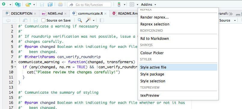
Praktikum: Code-Style

Den Code in eine neue Quarto-Datei formatieren:

library( palmerpenguins )
library(tidyverse   )

penguins|>filter( species=="Adelie" )|>group_by(island)|>summarize(n=n(),mean_bill=
mean(bill_length_mm,na.rm=TRUE))|>filter(n>10)

penguins|>filter(   species=="Chinstrap",island%in%c("Dream","Biscoe"),flipper_length_mm>190,
body_mass_g<4000)|>group_by(sex)|>summarize(
mean_mass=mean(body_mass_g,na.rm=TRUE),count=n())|>filter(count>5)

10:00

Danke! 🌔

Slides created via revealjs and Quarto.

Access slides as PDF.

All material is licensed under Creative Commons Attribution Share Alike 4.0 International.